• Produktbild: Finite Elements Using Maple
  • Produktbild: Finite Elements Using Maple

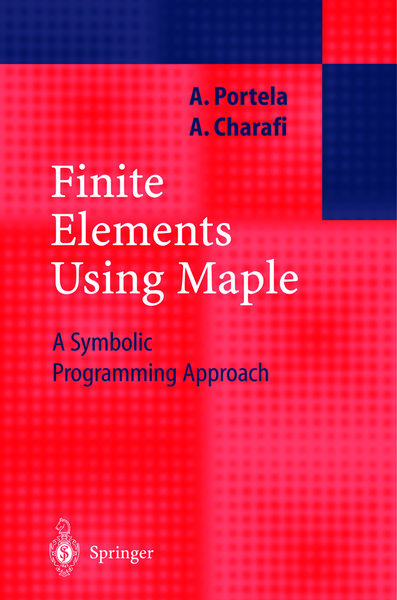
Finite Elements Using Maple A Symbolic Programming Approach

Fr. 73.90

inkl. gesetzl. MwSt., Versandkostenfrei


Beschreibung

Produktdetails

Einband

Taschenbuch

Erscheinungsdatum

27.10.2012

Verlag

Springer Berlin

Seitenzahl

326

Maße (L/B/H)

23.5/15.5/1.9 cm

Gewicht

522 g

Auflage

Softcover reprint of the original 1st ed. 2002

Sprache

Englisch

ISBN

978-3-642-62755-2

Beschreibung

Rezension

From the reviews:

"The purpose of this book is to illustrate how the computational environment of Maple can be used in a finite element ... . It gives to the reader a very unique insight into the finite element method together with symbolic programming approach ... . In summary, this book is an excellent introductory book for finite element method and I strongly recommend to all undergraduate and postgraduate students and also to engineers and scientists who wish to program easily the finite element method." (T.E. Simos, Journal of Computational Methods in Sciences and Engineering, Vol. 3 (2), 2003)

"This book is an essential tool written to be used as the primary text for an undergraduate or early postgraduate course as well as a reference book for engineers and scientists who want to develop quickly finite-element programs." (European Journal of Mechanical and Environmental Engineering, Vol. 47 (2), 2002)

Produktdetails

Einband

Taschenbuch

Erscheinungsdatum

27.10.2012

Verlag

Springer Berlin

Seitenzahl

326

Maße (L/B/H)

23.5/15.5/1.9 cm

Gewicht

522 g

Auflage

Softcover reprint of the original 1st ed. 2002

Sprache

Englisch

ISBN

978-3-642-62755-2

Herstelleradresse

Springer-Verlag KG
Sachsenplatz 4-6
1201 Wien
AT

Email: GPSR Kontakt

Noch keine Bewertungen vorhanden

Verfassen Sie die erste Bewertung zu diesem Artikel

Helfen Sie anderen Kundinnen und Kunden durch Ihre Meinung.

Kundinnen und Kunden meinen

Bewertungen (0)

  • Produktbild: Finite Elements Using Maple
  • Produktbild: Finite Elements Using Maple
  • 1. Introduction to Maple.- 1.1 Basics.- 1.2 Entering Commands.- 1.3 Fundamental Data Types.- 1.4 Mathematical Functions.- 1.5 Names.- 1.6 Basic Types of Maple Objects.- 1.6.1 Sequences.- 1.6.2 Lists.- 1.6.3 Sets.- 1.6.4 Arrays.- 1.6.5 Tables.- 1.6.6 Strings.- 1.7 Evaluation Rules.- 1.7.1 Levels of Evaluation.- 1.7.2 Last-Name Evaluation.- 1.7.3 One-Level Evaluation.- 1.7.4 Special Evaluation Rules.- 1.7.5 Delayed Evaluation.- 1.8 Algebraic Equations.- 1.9 Differentiation and Integration.- 1.10 Solving Differential Equations.- 1.11 Expression Manipulation.- 1.12 Basic Programming Constructs.- 1.13 Functions, Procedures and Modules.- 1.14 Maple’s Organization.- 1.15 Linear Algebra Computations.- 1.16 Graphics.- 1.17 Plotter: Package for Finite Element Graphics.- 1.17.1 Example.- 1.17.2 Example.- 1.17.3 Example.- 2. Computational Mechanics.- 2.1 Introduction.- 2.2 Mathematical Modelling of Physical Systems.- 2.3 Continuous Models.- 2.3.1 Equilibrium.- 2.3.2 Propagation.- 2.3.3 Diffusion.- 2.4 Mathematical Analysis.- 2.5 Approximation Methods.- 2.6 Discrete Models.- 2.7 Structural Models.- 3. Approximation Methods.- 3.1 Introduction.- 3.2 Residuals.- 3.3 Weighted-Residual Equation.- 3.3.1 Example.- 3.4 Approximation Functions.- 3.5 Admissibility Conditions.- 3.5.1 Example.- 3.6 Global Indirect Discretization.- 3.6.1 Satisfaction of Boundary Conditions.- 3.6.2 Domain Methods of Approximation.- 3.6.3 Galerkin Method.- 3.6.4 Least Squares Method.- 3.6.5 Moments Method.- 3.6.6 Collocation Method.- 3.6.7 Example.- 3.6.8 Example.- 3.7 Integration by Parts.- 3.7.1 Strong, Weak and Transposed Forms.- 3.7.2 One-Dimensional Case.- 3.7.3 Example.- 3.7.4 Higher-Dimensional Cases.- 3.7.5 Example.- 3.8 Local Direct Discretization.- 3.8.1 Nodes and Local Regions.- 3.8.2 Satisfaction of Boundary Conditions.- 3.8.3 Finite Difference Method.- 3.8.4 Finite Element Method.- 3.8.5 Boundary Element Method.- 3.8.6 Example.- 3.8.7 Example.- 3.8.8 Example.- 4. Interpolation.- 4.1 Introduction.- 4.2 Globally Defined Functions.- 4.2.1 Polynomial Bases.- 4.2.2 Example.- 4.2.3 Example.- 4.2.4 Conclusions.- 4.3 Piecewisely Defined Functions.- 4.3.1 Spline Interpolation.- 4.3.2 Finite Element Interpolation.- 4.4 Finite Element Generalized Coordinates.- 4.4.1 Convergence Conditions.- 4.4.2 Geometric Isotropy.- 4.4.3 Finite Element Families.- 4.5 Finite Element Shape Functions.- 4.5.1 Natural Coordinates.- 4.5.2 Curvilinear Coordinates.- 4.5.3 Example.- 4.6 Parametric Finite Elements.- 4.7 Isoparametric Finite Elements.- 4.7.1 Convergence Conditions.- 4.7.2 Evaluation of Element Equations.- 4.7.3 Numerical Integration.- 4.8 Linear Triangular Isoparametric Element.- 4.8.1 Example.- 4.8.2 Example.- 4.8.3 Example.- 4.8.4 Example.- 5. The Finite Element Method.- 5.1 Introduction.- 5.2 Steady-State Models with Scalar Variable.- 5.2.1 Continuous Model.- 5.2.2 Weighted Residual Galerkin Approximation.- 5.2.3 Discrete Model.- 5.3 Finite Element Mesh.- 5.3.1 Linear Triangular Isoparametric Element.- 5.3.2 Total Potential Energy.- 5.3.3 Internal Potential Energy Density.- 5.3.4 Mesh Topology.- 5.4 Local Finite Element Equations.- 5.5 Global Finite Element Equations.- 5.6 Exact Boundary Conditions.- 5.7 Solution of the System of Equations.- 5.8 Computation of Derivatives.- 5.9 Finite Element Pre- and Post- Processing.- 5.10 Cgt-fem: Package for Finite Element Analysis.- 5.10.1 Data Preparation.- 5.11 Example.- 5.12 Example.- 5.13 Example.- 5.14 Example.- 6. Fluid Mechanics Applications.- 6.1 Introduction.- 6.2 Continuous Models of Fluid Flow.- 6.2.1 Incompressible Fluids.- 6.2.2 Inviscid Fluids.- 6.2.3 Irrotational Flows.- 6.2.4 Steady-State Flows.- 6.2.5 Bernoulli’s Energy Conservation.- 6.2.6 Velocity Potential.- 6.2.7 Stream Function.- 6.3 Confined Flows.- 6.4 Unconfined Flows.- 6.5 Groundwater Flows.- 6.5.1 Darcy’s Hypothesis.- 6.5.2 Dupuit’s Hypothesis.- 6.6 Example.- 6.6.1 Flow Under a Dam.- 6.6.2 Problem’s Solution.- 6.7 Example.- 6.7.1 Flow in an Unconfined Aquifer.- 6.7.2 Problem’s Solution.- 7. Solid Mechanics Applications.- 7.1 Introduction.- 7.2 Continuous Models.- 7.3 Fundamental Continuous Model: Elasticity Theory.- 7.3.1 Strain-Displacement Equations.- 7.3.2 Equilibrium Equations.- 7.3.3 Stress-Strain Equations.- 7.3.4 Boundary Conditions.- 7.3.5 Elastic Fields.- 7.3.6 The Work Theorem.- 7.3.7 Theorem of Virtual Displacements.- 7.3.8 Theorem of Total Potential Energy.- 7.4 Finite Element Model.- 7.4.1 Weighted Residual Equation.- 7.4.2 Theorem of Work.- 7.4.3 Theorem of Virtual Displacements.- 7.4.4 Discretization.- 7.5 Mesh Topology.- 7.5.1 Total Strain Energy.- 7.5.2 Distribution of the Strain Energy Density.- 7.6 Constrained Displacements.- 7.7 Application of the Finite Element Model.- 7.8 Three-Dimensional Equilibrium States.- 7.8.1 Constant-Strain Tetrahedron Element.- 7.9 Two-Dimensional Equilibrium States.- 7.9.1 Plane Stress and Plane Strain.- 7.9.2 Asymptotic Model: Plane Elasticity.- 7.9.3 Constant-Strain Triangular Isoparametric Element.- 7.9.4 Cst_fem: Package for Finite Element Analysis.- 7.9.5 Data Preparation.- 7.9.6 Example.- 7.9.7 Example.- 7.9.8 Example.- 7.9.9 Example.- 7.10 One-Dimensional Equilibrium States.- 7.10.1 Asymptotic Model: Theory of Bars.- 7.10.2 Truss Element.- 7.10.3 Skew Elements.- 7.10.4 Beam Element.- 7.11 Further Study.